New Generation Activity-Based Travel Demand Models: From Trips To Lives

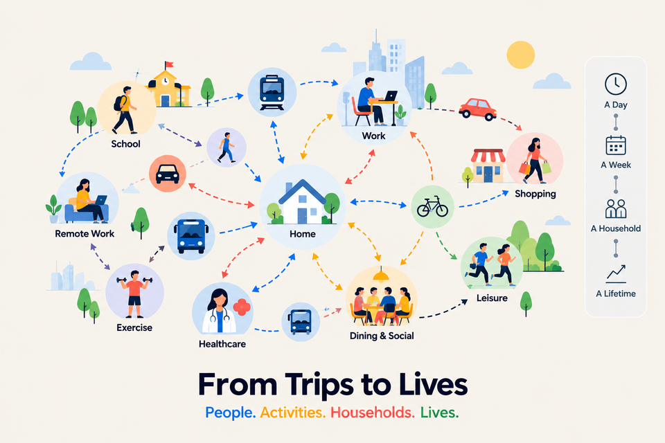
For decades, transportation planning has relied on models that simplify an extraordinarily complex question:

How will millions of different people respond when we change the transportation system?

A new generation of travel demand modeling is pushing toward much greater behavioral detail.

​Instead of representing populations primarily through aggregate groups and snapshots, researchers are developing complex synthetic populations that can evolve over time, incorporate household and social relationships, and feed into increasingly sophisticated activity-based models.

​At the same time, advances in discrete choice modeling and computation are making it possible to model decisions involving enormous numbers of alternatives—bringing travel demand models closer to the complexity of the choices people actually face.

​What does this mean for the future of transportation modeling?

At Mobility Forum, I spoke with Michel Bierlaire, Professor at EPFL, about this new generation of disaggregate travel demand models. This memo is a deep dive of our discussion on three questions:

1. The four big shifts that are changing travel demand modeling: from modeling trips to understanding people’s days, households, and lives
2. How can we model the enormous complexity of people’s daily choices, relationships, and lives? Once we model human behavior in this much detail, the number of possible choices explodes into the billions. How do we make that computable, what data do we need, and how do we know the results are good enough?
3. What does all of this mean for transportation planners? How Swiss Railways put these ideas to work, and what MPOs, DOTs and transportation authorities should consider as they make their next modeling investments.

Part 1. Why a New Generation of Travel Demand Models? Four Shifts in Behavioral Complexity.

The value of richer models lies in the scope of questions they can address, not in predictive precision. The added detail captures behavior relevant to the planning and investment decision.

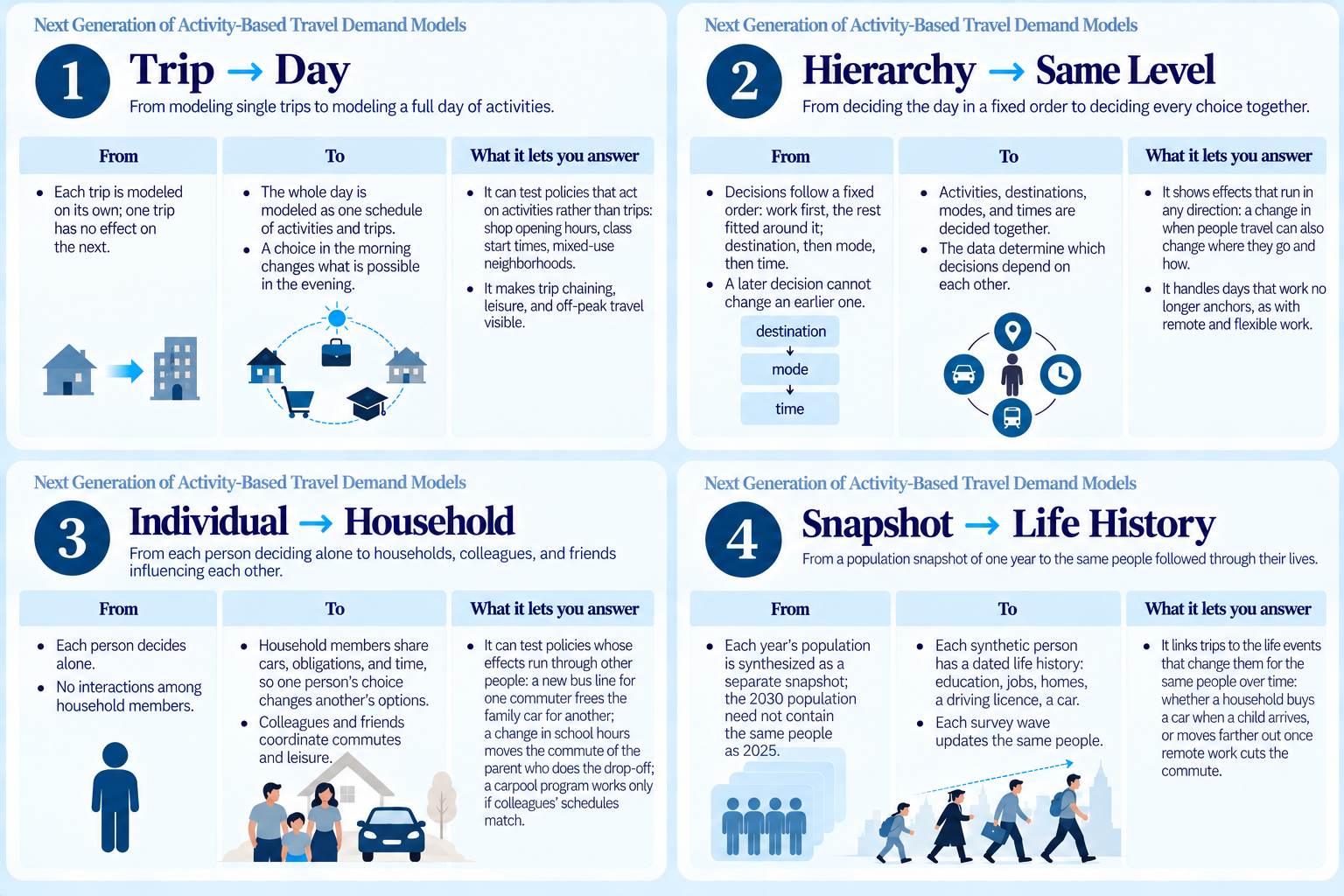
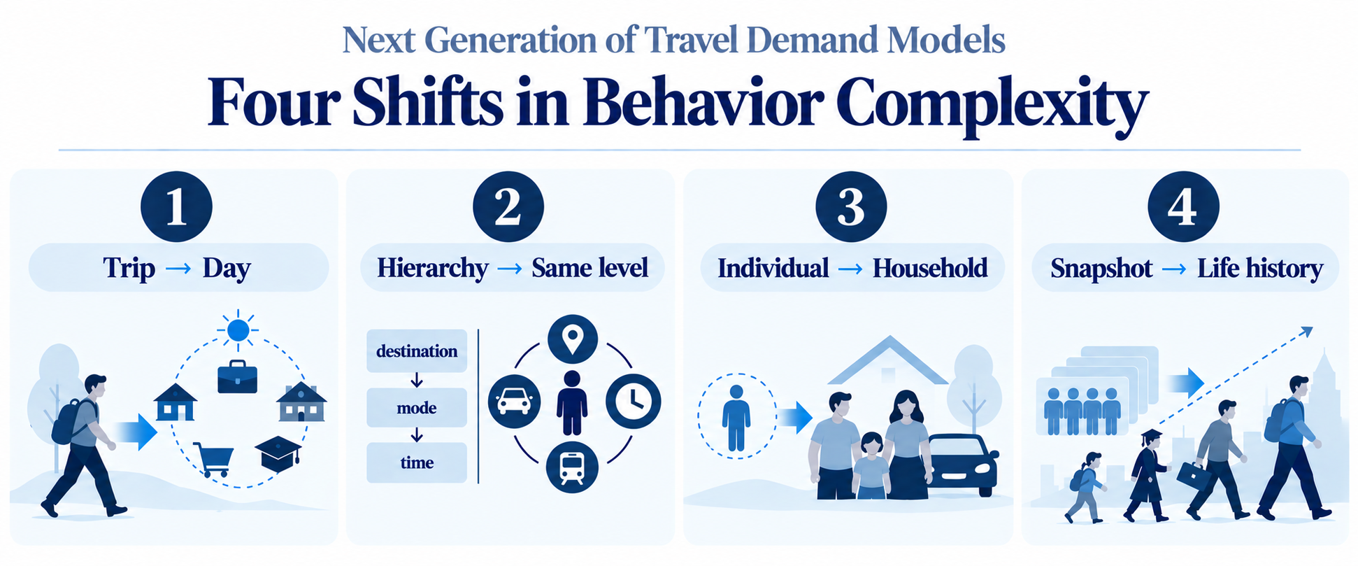
Complexity Shift 1: From Modeling Single Trips to Modeling An Entire Day

Three questions a trip-based model cannot answer:

1.  Remote work changes where activities take place, when people travel, and how the rest of the day is organized.

2.  At EPFL and the university next door, classes start at the same time, and the public transportation operator asked whether EPFL could shift its start time to spread the morning peak.

3. In Switzerland the cantons set shop closing times by law, typically between 18:30 and 20:00 on weekdays with Sundays closed, and voters have repeatedly refused to loosen them. What would a later closing hour do to the evening peak?

Answering these questions requires the model to represent the day that the policy changes: the activities, when and where they happen, and the constraints that bound how the rest of the day can adjust. A trip table has none of that. A commute removed by remote work reorganizes the day rather than subtracting a journey; a later start or a later closing hour moves the activities before and after it, and the peak spreads, or moves to another hour or another place.

Travel serves activities, and activity-based models reconstruct the travel needed to accomplish them.

Someone might shorten lunch to finish work earlier and play tennis in the evening. Each choice changes what remains possible later, and modeling the trips separately misses the time allocation that connects them.

A full-day schedule makes these connections explicit. Preferences matter, but so do constraints: a day contains 24 hours, some activities are mandatory, and a car may be unavailable. The model represents both what a person wants and what that person can do. Looking across the full day also brings leisure and off-peak demand into view.

The approach has existed since the late 1990s; the frontier is how completely the activities and their connections are represented.

Complexity Shift 2: From an Assumed Decision Hierarchy to Decisions On the Same Level

The 1990s’ activity-based models manage complexity by arranging choices in sequence: primary activities first, then secondary activities, destinations, and modes.

Each step is manageable, but the sequence dictates which decisions come first. In reality, most of the time it is a joint decision.

This decision hierarchy was shaken by COVID and working from home. The commuting trip may no longer be the anchor of a day. In Switzerland, leisure, not work, is already the largest trip purpose according to census.

The new approach places the decisions on the same level. Constraints define the feasible schedules, preferences rank them, and observed behavior shows how the choices fit together. Letting the data decide means not prescribing a decision order in advance.

This is not a claim about the psychological process. People do not enumerate every possible day, and each person decides differently. The objective is only to predict behavior under specified conditions while avoiding a hierarchy that may be wrong.

Complexity Shift 3: From the Isolated Individual to Households and Social Networks

A person’s feasible day depends on other people. In a household with one car, one member’s decision to drive removes that option for another. Someone must take the children to school. We want to enjoy dinner together. Shared resources and obligations make individual choices interdependent.

Joint activities require compatible arrival times. Shared cars and shared obligations are shared constraints. And the outcome is bargained among the members, not chosen by one of them.

These interactions change both constraints and objectives. A household member may accept an inconvenient trip to improve someone else’s day, which a model of individuals maximizing personal convenience misses.

The model must consider compatible combinations of schedules across people.

Beyond the household, colleagues coordinate commutes and friends coordinate leisure. Identifying the relevant relationships is part of understanding demand. Attitudes and perceptions matter too: people respond to perceived service quality, which differs from measured conditions.

Complexity Shift 4: From a Static Population Snapshot to Synthetic Population with Life Histories

Important life decisions such as moving home, changing jobs, forming a family, and buying a car shape daily travel over years.

A travel model carries those choices in its synthetic population: artificial individuals who reproduce the statistical population without corresponding to any real person, on which the activity models run. Built as a snapshot, that population knows nothing of the years behind it.

Separate snapshots lack continuity. A population synthesized for 2025 and another for 2030 may each match its year’s statistics without representing the same people.

The alternative is to synthesize whole life histories dated: birth, education, work, residence, driving license, car ownership. The same person is then followed from one survey to the next.

The key moments are the ones that trigger many later decisions. When people move, they decide whether to live near transit and how many cars to own, and those arrangements persist for years. Remote work changes the trade-off between commute distance and frequency: a more distant home becomes attractive when the commute is less frequent.

The life history of shift 4 fixes where someone lives and works and whether a car is available, and shifts 1 to 3 decide the day inside those constraints. Remote work is the one place where the day reaches back into the life.

Part 2. Managing the Explosion of the Choice Set: Method, Data, Validation

Richer representation is only useful if it can be computed, fed by data, and checked. All four shifts expand the choice set, and they compound.

A single trip involves a handful of modes, and a destination choice model may have a few hundred options. A full day schedule adds which activities to perform, in what sequence, where, when, for how long, and by what mode, and the combination quickly explodes.

Removing the hierarchy removes the pruning: a model that fixes primary activities before secondary ones never considers most combinations, while a model that decides everything at the same level keeps all of them in the choice set.

Households multiply again, because only compatible combinations of members’ schedules are feasible, and feasibility depends on shared cars, shared obligations, and shared arrival times.

Life histories add sequences of events over decades: where someone lived, worked, and studied, and when.

Three shifts grow the day; one grows the population, and it runs first. Each object has its own machinery, its own data, and its own test.

The Technical Core: Formulate- Optimize - Simulate - Estimate

Listing billions of combinations is impractical. Discrete choice modeling supplies a theory of preferences and probabilistic behavior, and methods for learning from observed choices.

Combinatorial optimization supplies ways to describe and search enormous sets of feasible alternatives. It is the same mathematics behind timetabling, vehicle routing, and airline operations.

A day, in what follows, means a full daily schedule: which activities, where, when, for how long, by what mode. Four moves connect discrete choice and optimization.

Formulate codifies the rules that define the feasible set. Instead of listing every feasible day, write the rules, the constraints a feasible day must satisfy: 24 hours, mandatory activities, a car or no car, set by the life history. An objective function represents preferences. Constraints plus preferences form an optimization problem. The behavioral relationships stay in the rules; no list of alternatives is ever written.

Households enter here. Shared cars and shared obligations are written as constraints across the members’ schedules, and the structure they add is what the search exploits. How to write a household’s preferences remains contested: published formulations sum the members’ utilities, or maximize the best-off or the worst-off member, and the framework accepts any of them without settling how families negotiate. Attitudes enter the utility through hybrid choice models with latent variables, whenever suitable data exist.

Optimize identifies the best day schedule by searching the space efficiently. Branch-and-bound divides the problem into slices and uses bounds to discard slices that cannot contain the best solution. Standard solvers, Gurobi and CPLEX, came first; decomposition methods, Benders decomposition and column generation, now break the model into easier sub-models. The successes in optimization come from adapting algorithms to the structure of the problem, here specific people with specific interactions, rather than from off-the-shelf tools.

Simulate adds random utility, from one day to a distribution. A deterministic optimization yields one preferred schedule. Random utility adds variation: draw realizations of the random components, solve the optimization for each draw, and repeat, perhaps thousands of times. The result is a distribution of schedules. The draws are independent and run in parallel, but the computation remains demanding.

Estimate identifies preference parameters from sampled alternatives. Estimation needs alternatives to compare with the schedule someone actually followed. Markov chain Monte Carlo methods, Metropolis-Hastings in particular, draw alternatives from the combinatorial space, and draw them where it matters: most of the billions are irrelevant because they would never be attractive, and the informative ones are those competing with the observed choice. Sampling only where it matters introduces a known bias, which importance-sampling corrections remove in estimation.

The four moves form two loops. Formulate is the hinge: its rules and its utility feed both loops.

The predict loop runs Formulate, Optimize, and Simulate, once per scenario. Formulate writes the rules and the objective for the scenario: a later start time, a later closing hour, a new line. Optimize returns the best schedule for one draw of the random utility. Simulate repeats the draw and the solve, thousands of times per person. The result is a distribution of schedules for each person and, summed across the population, the demand the scenario produces.

The learn loop runs Formulate and Estimate once. The same rules and utility, with starting parameters, go to a sampler, which prepares each observed person’s competitive alternatives, and Estimate compares the schedule actually chosen with them. The estimated parameters go into the objective; the rules are unchanged; then the predict loop runs with them.

Estimate’s alternatives do not come from Simulate, and for a reason: Simulate produces the schedules the estimated model predicts, and estimating the parameters on the model’s own predictions would be circular. The sampler draws alternatives from the feasible set instead, and the sampling is corrected so the estimates stay unbiased.

The Population's Machinery: Prior and Update

A demographic model supplies the life course, each survey wave corrects it, and the result is one population followed over years

The population is built in two layers.

Demographic models of how a population evolves supply the prior: when people are born, study, start work, move, obtain a licence, acquire a car.

Bayesian updating against each survey wave corrects it, in Switzerland the mobility microcensus, taken every five years. Cross-sectional data collected at several points in time thereby yield a longitudinally coherent population: snapshots extracted from different years refer to the same individuals, which gives researchers longitudinal synthetic data that no survey collected.

The update is bounded by the prior. It corrects what the prior allows to vary and cannot put back what the prior excludes. In the Swiss application, the prior assumed that 85 percent of everyone eventually obtains a driving licence, whatever their sex or generation; the 2010 microcensus showed 89 percent of men and 75 percent of women, because many older women never did. The updated population gave 78 percent for both: the total was close, and the relationship between licence and sex had the wrong sign, because the prior had no place for it. The remedy is in the prior, letting the chance of ever holding a licence depend on birth cohort and sex.

The histories are modeled constructions. A synthetic history that matches the statistics does not say why a person moved or changed jobs. A policy meant to change those decisions, a housing subsidy or a new transit line, acts on the why, and a population that only reproduces the pattern cannot show the response.

From Algorithms to the Data Frontier

The data record where people went; the model needs why, and what else they could have done

Better algorithms increase what can be represented. A model that decides the whole day at once needs to know the whole day: the activities, the constraints, and the alternatives that were open. That is where the data run out.

The typical data are travel diaries and time-use records, which connect movement to activities. Switzerland’s mobility microcensus is one, and phones now help respondents reconstruct their day with less effort.

Social relationships are harder. Census data report household composition, but friendships and colleague relationships require dedicated collection. Snowball sampling, in which respondents name contacts who are then approached, reveals connections at the cost of a strong selection bias. Online friendship is not the same as the friendship that shapes shared travel.

GPS traces, smart cards, connected vehicles, and transactions record extensive movement: where people went, when, how often, and at a scale no survey reaches. They are useful for the movement side and limited for the choice side, because they record neither the activity’s purpose, nor the constraints on the alternatives, nor why someone declined an option. Transportation research is data-rich and data-poor at the same time.

Two rules follow: start with the research question rather than the dataset, and fuse sources rather than rely on one. Privacy limits access as well. Detailed location histories reveal homes and workplaces even without names, and in Europe, under the General Data Protection Regulation (GDPR), the legal obstacles to using them have grown over the past five years.

Is Synthetic Population Good Enough?

It is good enough if it does what it is supposed to do.

Reproducing the real population is not the goal. If it were, the real population would do, and the synthetic one exists precisely so that no real person is in the data. There is therefore no held-out real population to reproduce, and out-of-sample validation in the regression sense does not apply. The test is different in kind, and it comes in three steps.

Sanity checks come first: the marginal distributions and the main correlations that matter for the question should match the real population, and the whole should make sense.

Then come objective-based tests. Use the population in the scenarios it exists for, in a traffic simulator or an activity model, and check whether it captures the heterogeneity that matters. Vary something and check whether the population is still relevant: a robustness test rather than a fit statistic.

If it is not detailed enough for the question, refine it. The model is relevant only in the context where it is used, and no single fit statistic serves every purpose.

Behavioral predictions are validated separately. With cross-sectional data, the traditional test holds out a share of the observations, say 20 percent, re-estimates on the rest, and predicts the held-out share. With panel data, the model is estimated on earlier years and run forward, a backcast; such data are rare.

Agencies should say what they expect to validate: population characteristics, observed behavior, or performance over time. Success on one does not establish the others.

Part 3. From Research to Application: Swiss Railways

Swiss Federal Railways (SBB) faces an interesting problem: Peak-hour trains are packed. Yet across the full day, the railway uses only about 28% of its capacity.

So how to bring more passengers onto trains during off-peak hours? The goal is to understand the full chain of activities and trips so that the railway can make long-term infrastructure and service decisions. For example, Swiss Railways has considered what would happen if trains operated more like a metro, with service on every line perhaps every 15 minutes.

SBB can’t answer that by looking at train trips alone. They need to understand people’s entire day and activities behind it - not just commuting. Why are they traveling? What are they doing before and after the train ride? How do they get to the station? What happens if service changes?

SBB had already built its own activity-based model and uses MATSim to understand these broader travel patterns. Michel and his team worked with Swiss Railways to test their newer methodology—using combinatorial optimization to handle the enormous number of possible activity and travel choices within the railway’s existing modeling tool. The project was successful: the model reproduced the observed distribution of activities satisfactorily.

The results successfully reproduced observed activity patterns.

Swiss Railways understood the value of activity-based modeling. New modeling methods become useful when they meet a real planning question, an existing modeling foundation, and an agency capable of using the results. The new methodology added capability where it mattered.

What should MPOs, DOTs and transportation agencies do?

Do not do a head-to-head comparison of a four-step and an activity-based model on the same question as the two answer different questions. Traditional models may remain appropriate for the questions they were built for. Start by reviewing what the newer models can do and judge whether that is relevant to your questions. More elaborate models earn their place through the questions they can address and the quality of the resulting analysis. Connect activities, people, and time, decide them together, and the model shows what a policy does to people's lives, not only to trips.

For an agency planning its next investment, I suggest five steps:

1. start with a question the present system handles poorly;
2. identify the behavioral relationships needed to answer it and the evidence available;
3. pilot the capability within a defined planning task, with explicit criteria for whether it improves the analysis;
4. invest in staff who can explain the assumptions and maintain the model after the project ends;
5. and weigh the burden against the policy value, because data collection, calibration, computation, and interpretation consume resources, and a focused application shows which detail matters before a broader rebuild.

— Jinhua

Listen to our full 46 mins conversation on Mobility Forum Podcast: